Quickstart

This guide walks through what each section of notebooks/msm_notebook.ipynb does, what options you can tune, and what outputs to expect. For input-file formatting rules, see Data Layout. For argument-by-argument details of the main Python functions, see Function Reference.

Before you start

Clone the repository:

git clone https://github.com/fberkemeier/MultiLayer-NotchDelta.git

From the repository root:

pip install -r requirements.txt
jupyter notebook notebooks/msm_notebook.ipynb

Detailed walkthrough

1. Dependencies and MSM import

This section imports standard scientific Python libraries and then imports functions from src/msm_model.py. Use this as a quick sanity check: if import fails here, fix environment/dependency issues before running analysis cells.

2. Data setup and region selection

This section defines which datasets to run and builds all dictionaries used later.

Typical pattern:

wing_regions = ['wd_1', 'wd_2', 'wd_3']

wing_discs = list_wing_discs(wing_regions)
signalling_labels_dict = load_signalling_labels_dict(wing_regions)
wd_dict = build_wd_label_dict(wing_regions)
gap_dict = build_gap_dict(wing_regions)
n_dict = build_n_layers_dict(wing_regions)
heights_dict = build_default_height_dict(wing_regions)

A_dict = build_adjacency_dict(wing_regions)
centroids_dict = build_centroids_dict(wing_regions)
area_apical_dict = build_area_apical_dict(wing_regions)
diam_apical_dict = build_diam_apical_dict(wing_regions)

Key options in this section:

• wing_regions: controls which region files are loaded and analyzed.

• notch_data: user-owned intensity profile array (editable per dataset).

• heights_dict: can use metadata defaults or values derived from height_set.

If this section fails, the most common cause is mismatched names between wing_region_metadata.csv and file names in data/.

3. Single simulation (graph plot)

This subsection sets model parameters and runs one call to compute_band_distance for a selected region. It is the best entry point to validate that your data and parameters produce expected spatial patterns.

Main parameters users typically change:

• wing_region: which dataset to run.

• Lmax: signalling depth cutoff.

• omega_type: depth-weight function (exp, cnt, lin, exp0).

• k, h, Ka, Kr, nu: Notch-Delta model parameters.

• alpha: straightening level for non-apical contacts.

• graphsaveQ: whether to save the graph image to figures/.

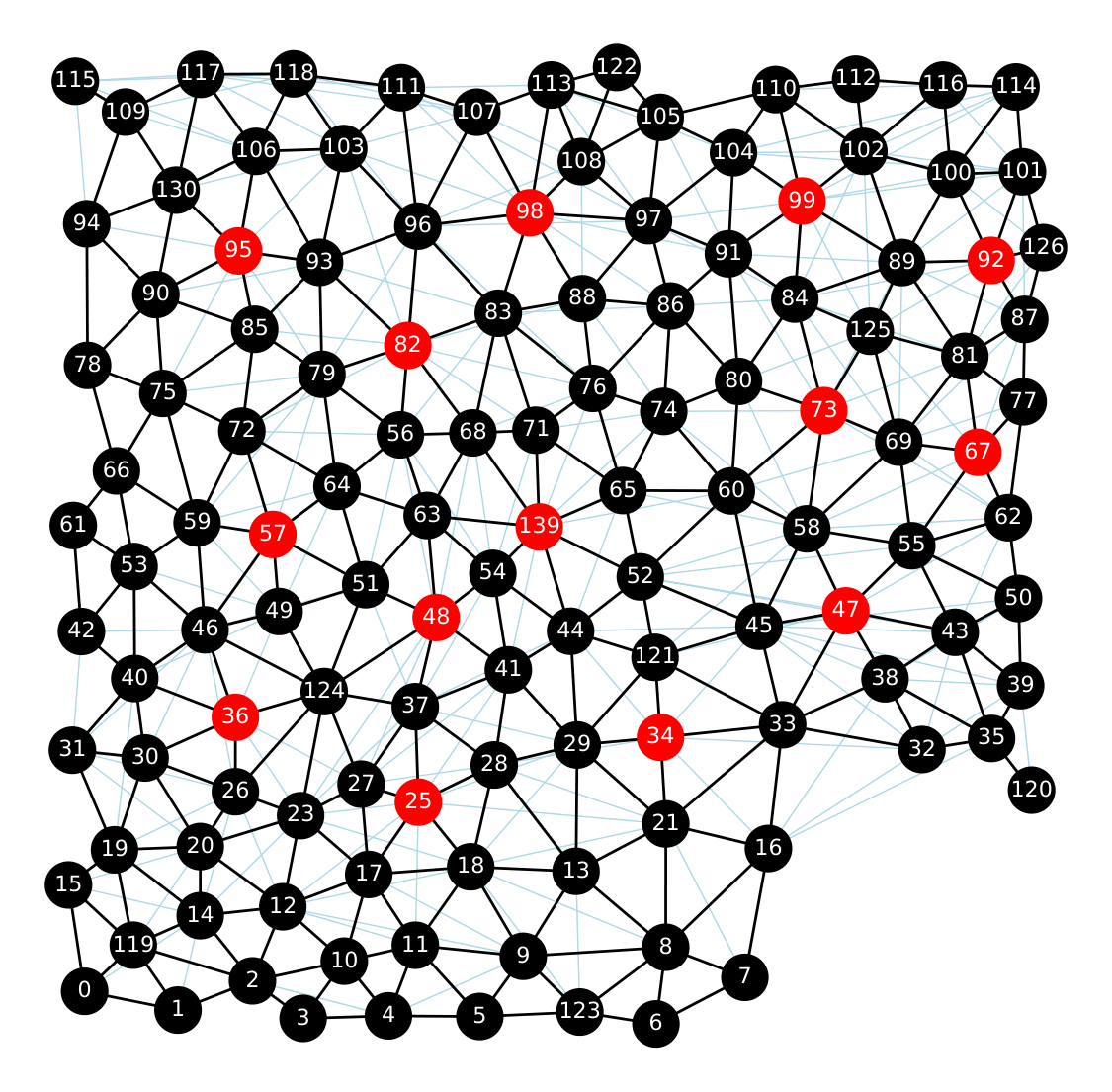
MSM simulation over a wing disc. SOP cells are displayed in red (high Delta).

4. SOP spacing plots

This subsection sweeps depth values (Lmax_list) and computes spacing statistics across selected regions. It is used to quantify how signalling range affects spacing robustness and degeneracy.

You can control:

• spsteps: number of sampled depth points.

• threshold: SOP threshold used for classification.

• normalQ: normalize depth weights to a common support.

• sim_number: number of repeated simulations per condition.

• plotting style through fancy_plot parameters.

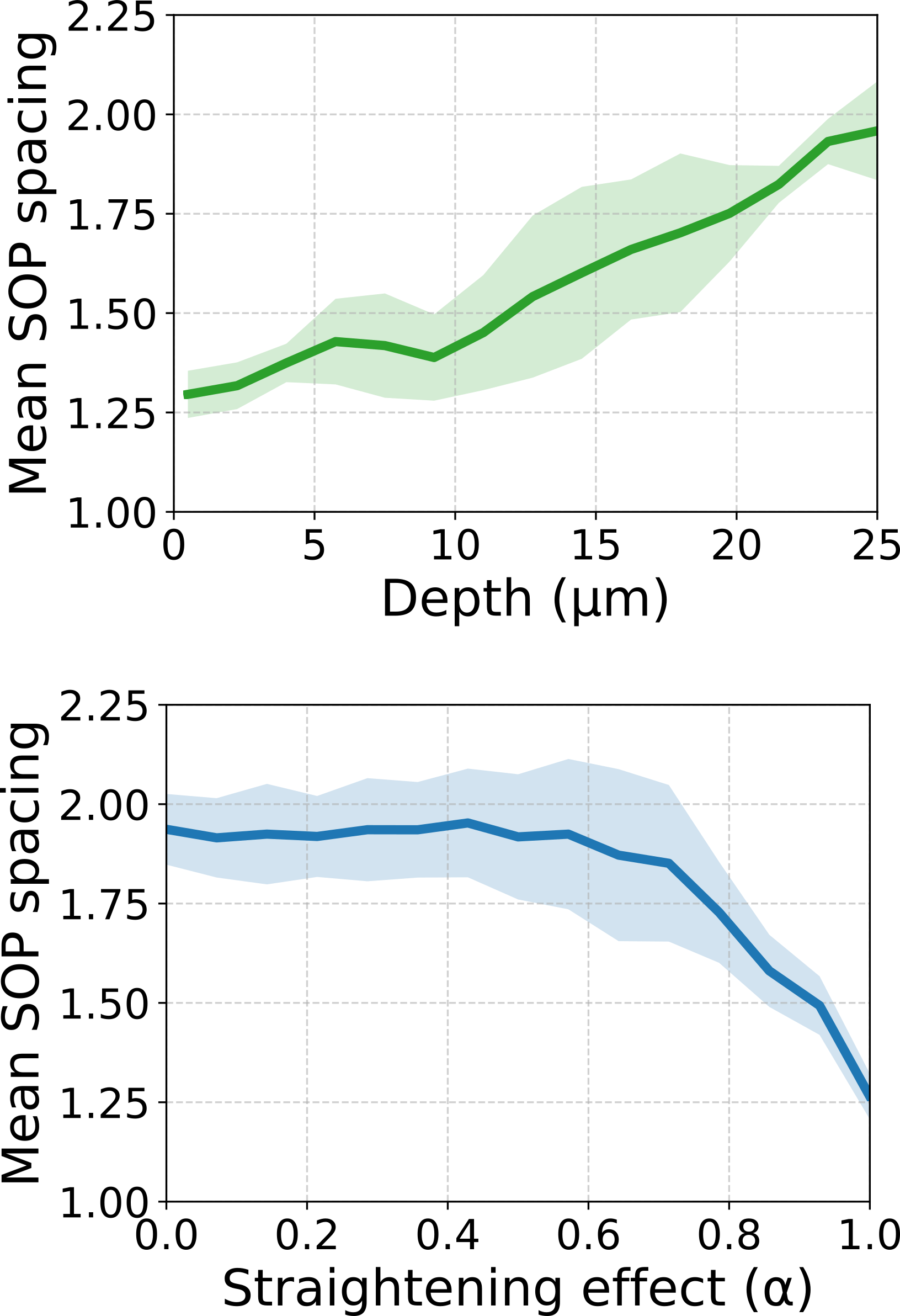
SOP spacing vs depth and straightening for 3 wing discs (wd_1, wd_2, and wd_3).

5. Other analyses

This final section contains complementary analyses:

• 3D neighbour counts: tests how non-apical connectivity changes under straightening (alpha sweep).

• Notch intensity fitting: fits an exponential profile to measured Notch data.

• Signalling weight histograms: visualizes integrated layer weights omega_k by region.

These analyses are useful for mechanistic interpretation and parameter diagnostics before running larger sweeps.

Practical usage patterns

• Run one region first (for example ['wd_1']) to validate data and runtime.

• Keep randomQ=False when you want deterministic debugging runs.

• Enable save flags only once plots look correct to avoid clutter in figures/.